Lambert W Function Implementation

The Matlab function lambertw included in this package is a self-contained M-function implementing the Lambert W function, also known as the Ω function or “product log.” It is equivalent to the numerical mode of the Symbolic Math Toolbox’s lambertw, however, no toolboxes are required to use this function.

License (BSD)

Function Use

w = lambertw(z) computes the principal value of the Lambert W function, \(W_0\). The input z may be a complex scalar or array. For real z, the result is real on the principal branch for z ≥ −1/e.

w = lambertw(b,z) specifies which branch of the Lambert W function to compute. If z is an array, b may be either an integer array of the same size as z or an integer scalar. If z is a scalar, b may be an array of any size.

Background

The Lambert W function is defined as the function W(z) such that

\[ W(z) \mathrm{e}^{W(z)} = z \]

for all complex values z. As log z is the inverse of e^z, W(z) is the inverse of z e^z. Like the complex logarithm, the Lambert W function is multivalued with a countably infinite number of branches. The branches are enumerated by the integers and are conventionally denoted by \(W_k\) for the kth branch.

The principal branch, \(W_0(z)\), is real-valued for −1/e ≤ z. If −1/e ≤ z < 0, then the branch \(W_{-1}(z)\) is also real-valued. In the complex plane, a surface plot of \(|W_0(z)|\) is

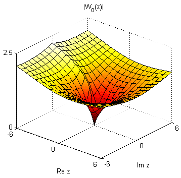
x = linspace(-6,6,51);
y = linspace(-6,6,51);
[x,y] = meshgrid(x,y);
w = lambertw(x + i*y);

surf(x,y,abs(w));
axis([-6,6,-6,6,0,2.5]);
view(40,32);
xlabel('Re z');
ylabel('Im z');
title('|W_0(z)|');

Algebra with the Lambert W Function

Although the Lambert W function may not be so widely known as the inverse trigonometry functions, it has essentially the same purpose as acos, asin, etc. as a building-block tool for solving equations. Generally, the goal is to manipulate all occurrences of the unknown variable x into an expression of the form \(f(x) \mathrm{e}^{f(x)}\), and then apply the Lambert W function.

Problem 1. Solve \(y = (x − 1) \mathrm{e}^{2x}\) for x.

Solution: The right-hand side is close to the necessary form \(f(x)\mathrm{e}^{f(x)}\), but some manipulation is necessary to change the factor \((x - 1)\) and the exponent 2x into the same expression. Multiplying both sides by 2,

\[2y = (2x - 2) \mathrm{e}^{2x}.\]

This form is closer, the exponent is only missing the −2. Multiplying both sides by e⁻² gets the desired form,

\[2\mathrm{e}^{-2}y = (2x - 2) \mathrm{e}^{2x-2}.\]

Now we can apply the Lambert W function to get

\[W(2\mathrm{e}^{-2}y) = 2x - 2,\]

which rearranges to the solution \(x = W(2\mathrm{e}^{-2} y)/2 + 1\). Note that since W is multivalued, the solution is multivalued; there are multiple values of x satisfying the equation.

Problem 2. Solve \(b^x = x^\alpha\) for x.

Solution: There is initially no visible instance of the exponential function, but rewrite \(b^x\) as \(\mathrm{e}^{x \log b}\) to reveal \[\begin{align} \mathrm{e}^{x\log b} &= x^\alpha \\ \mathrm{e}^{x(\log b) / \alpha} &= x. \end{align}\]

Now divide the exponential over to the right-hand side and multiply by \(-(\log b)/\alpha\):

The right-hand side is now in the form \(f(x)\mathrm{e}^{f(x)}\) where the Lambert W function can be applied:

\[W\bigl(-(\log b)/\alpha\bigr) = -x (\log b)/\alpha. \]

The solution is \(x = -(\alpha / \log b) W\bigl(-(\log b)/\alpha\bigr)\).

Problem 3. An old result [1] is the closed-form expression for iterated exponentiation:

\[z^{z^{z^\cdots}} = \frac{W(-\log z)}{-\log z}.\]

Find z such that \(z^{z^{z^\cdots}} = 2\).

Solution: Using the formula,

\[ -W(-\log z) / \log z = 2 \]

implies

\[\begin{align} W(-\log z) &= -2\log z \\ -\log z &= -2\log z \mathrm{e}^{-2\log z} \\ \mathrm{e}^{2\log z} &= 2 \\ z &= \sqrt{2}. \end{align}\]

Demos

The following command evaluates \(W_k(1)\) for \(k = -4,\ldots,4\):

w = lambertw((-4:4).',1)
w =

  -3.1630 -23.4277i
  -2.8536 -17.1135i
  -2.4016 -10.7763i
  -1.5339 - 4.3752i
   0.5671
  -1.5339 + 4.3752i
  -2.4016 +10.7763i
  -2.8536 +17.1135i
  -3.1630 +23.4277i

These values are all solutions of \(w\mathrm{e}^w = 1\). It is easy to verify numerically that they are solutions:

w.*exp(w)
ans =

   1.0000 - 0.0000i
   1.0000 - 0.0000i
   1.0000 + 0.0000i
   1.0000
   1.0000
   1.0000
   1.0000 - 0.0000i
   1.0000 + 0.0000i
   1.0000 + 0.0000i

Problem 3 in the previous section mentioned the formula for evaluating iterated exponentiation: \[z^{z^{z^\cdots}} = \frac{W(-\log z)}{-\log z}.\]

For example, set z = 1.3, then its iterated exponentiation is approximately zlim = 1.4710.

zlim = -lambertw(-log(z))/log(z)
zlim =

    1.4710

To verify this, computing z^z^z^...^z through 40 iterations shows that the iterated exponentiation does indeed converge to zlim.

zz(1) = z;
zlim = -lambertw(-log(z))/log(z);

for k = 1:40
   zz(k+1) = z^zz(k);
end

plot(zz,'.-');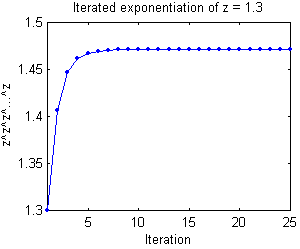

  k    zz     zlim-zz
  1  1.4065   0.065
  2  1.4463   0.025
  3  1.4615   0.0095
  4  1.4673   0.0037
  5  1.4696   0.0014
  6  1.4704   0.00055
  7  1.4708   0.00021
  8  1.4709   8.1e-005
  9  1.4710   3.1e-005
 10  1.4710   1.2e-005
 20  1.4710   8.9e-010
 30  1.4710   6.5e-014
 40  1.4710   2.2e-016

Test

Ideally, lambertw(b,z)*exp(lambertw(b,z)) = z for any complex z and any integer branch index b, but this is limited by machine precision. The inversion error |lambertw(b,z)*exp(lambertw(b,z)) - z| is small but worth minding.

Experimentation finds that the error is usually on the order of |z|×10⁻¹⁶ on the principal branch. This test computes the inversion error over the square [−10,10]×[−10,10] in the complex plane, large enough to characterize the error away from the branch points at z = 0 and −1/e.

N = 81;    % Use NxN points to sample the complex plane

R = 10;    % Sample in the square [-R,R]x[-R,R]
x = linspace(-R,R,N);
y = linspace(-R,R,N);
[xx,yy] = meshgrid(x,y);
z = xx + 1i*yy;

for b = -4:4
   w = lambertw(b,z);
   InvError = abs(w.*exp(w) - z);
   fprintf('Largest error for b = %2d:  %.2e\n',b,max(InvError(:)));
end

Largest error for b = -4:  2.51e-014
Largest error for b = -3:  2.39e-014
Largest error for b = -2:  1.39e-014
Largest error for b = -1:  7.94e-015
Largest error for b =  0:  5.40e-015
Largest error for b =  1:  7.94e-015
Largest error for b =  2:  1.39e-014
Largest error for b =  3:  2.39e-014
Largest error for b =  4:  2.51e-014

Implementation

The Lambert W function is implemented numerically with approximations from series expansions followed by root-finding. Depending on the desired branch and the proximity to the branch points at z = 0 and −1/e, different series expansions are used as initializations to the root-finder.

As developed in [2], lambertw uses Halley’s method, a fourth-order extension of Newton’s root-finding method. Convergence is very fast, usually requiring fewer than 5 iterations to reach machine accuracy.

References

[1] G. Eisenstein, “Entwicklung von α^α….” J. reine angewandte Math., vol. 28, 1844.
[2] R.M. Corless, G.H. Gonnet, D.E.G. Hare, G.J. Jeffery, and D.E. Knuth. “On the Lambert W Function.” Advances in Computational Mathematics, vol. 5, 1996.

Google Scholar LinkedIn